Connor Lynaugh Lab Reports

Lab 2 – IMU

Objective

The goal of this lab was to integrate the ICM-20948 IMU with the Artemis Nano and start collecting data on the car’s orientation using both accelerometer and gyroscope data. By combining sensor data and applying filters we are supposed to build a stable movement model that can be communicated over Bluetooth.

Setting up the IMU

The AD0_VAL in the Basic SparkFun Example dictates the least significant bit of the IMU’s I2C address and should be set to 1, which is default.

When moving the IMU, acceleration changes along the noted axes on the board, with gravity constantly applying acceleration towards the ground. If only moved in translational directions there are no gyroscope readings. The gyroscope only picks up rotational movements which rotate about the noted axes on the board. Similarly, rotational movements do not affect the accelerometer readings apart from the constant gravity.

To help with visual debugging I added a function which runs in the board setup and flashes the on-board LED three times before entering the main loop function.

Accelerometer

Using the equations from lecture I calculated pitch and roll using the accelerometer data in each axis. The trigonometric formulation uses atan2 to remain numerically stable across quadrants:

pitch = atan2(accX, accZ) * 180/M_PI;
roll  = atan2(accY, accZ) * 180/M_PI;

As shown in the video, the accelerometer is able to quickly follow changes in acceleration and, when stabilized, accurately display a large acceleration in the direction of gravity.

A Python script was written to parse and plot the data arrays sent from the Artemis over Bluetooth. The arrays sent for the accelerometer include time, pitch, and roll. An array size of 2000 accurately encompassed about 6-8 seconds of data.

The accelerometer showed overall good accuracy in all axes during repeated runs. The bias between a positive axis and a negative one was not substantial or consistent on reboot, so two point calibration was not required.

To test the noise levels of the IMU, the car motors were driven in its proximity and vibrations were induced on the testing table. The resulting noise levels were notably high across the whole spectrum once the data was analyzed in the frequency domain.

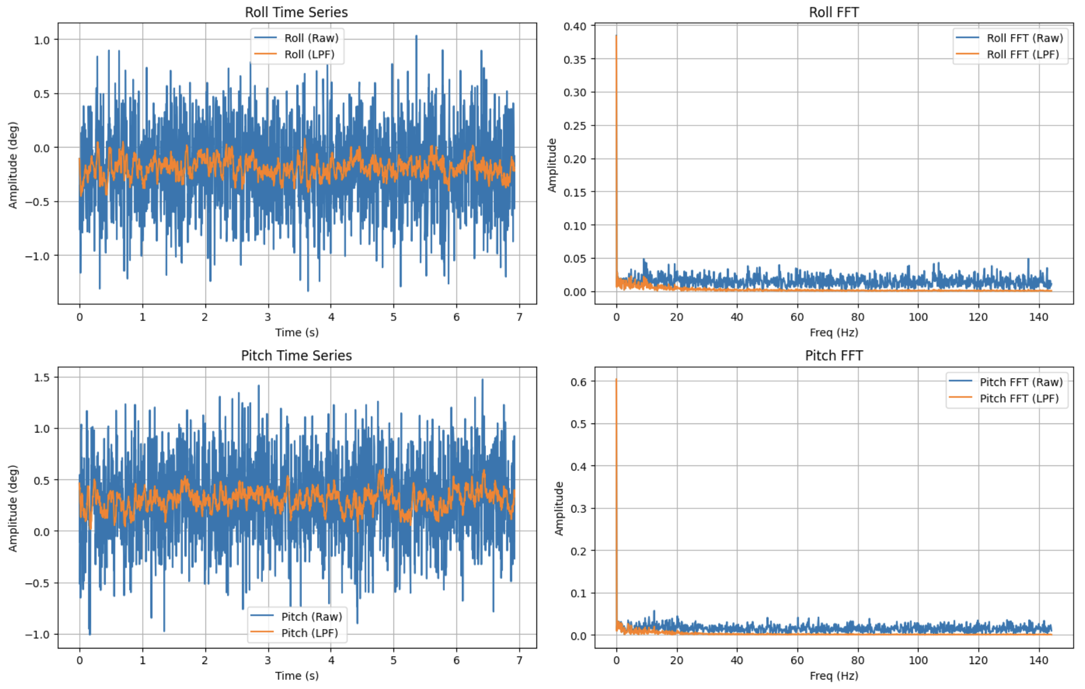
To better understand the accelerometer noise, I analyzed the recorded pitch and roll data in the frequency domain using a Fast Fourier Transform. This made it easier to separate useful motion from vibration, motor noise, and general sensor noise. The FFT showed that most of the useful accelerometer behavior was concentrated at low frequencies, especially below approximately 5 Hz. Higher-frequency components were less representative of the actual orientation of the car and more likely came from mechanical vibration and electrical noise.

Because of this, I chose a cutoff frequency of 5 Hz for the low-pass filter. This cutoff was a compromise between smoothness and responsiveness. A lower cutoff frequency would remove more noise, but it would also make the accelerometer angle respond too slowly to real movement. A higher cutoff frequency would make the signal more responsive, but would allow more vibration and noise to remain in the data. Since the robot’s orientation changes occur relatively slowly compared to the vibration noise, 5 Hz provided a reasonable balance.

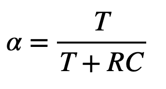
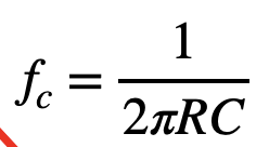
Using my measured sampling rate of approximately 288.66 Hz, this cutoff frequency produced an alpha value of 0.0982. In the filter implementation, each new filtered value is calculated as a weighted combination of the previous filtered value and the newest accelerometer reading. This means that sudden spikes in the accelerometer data have less influence on the final output, while consistent long-term changes in orientation are still preserved.

filtered_pitch = alpha * pitch + (1 - alpha) * previous_filtered_pitch;
filtered_roll  = alpha * roll  + (1 - alpha) * previous_filtered_roll;

After applying the low-pass filter, the accelerometer data became significantly smoother in the time domain and showed reduced high-frequency content in the frequency domain. Some noise still remained, but the filtered signal was much better suited for use in the complementary filter.

It is worth noting that the IMU board features an integrated Digital Motion Processor, or DMP, that can run its own algorithms on sensor feedback before passing the data to the Artemis board. However, for this portion of the lab I filtered the raw accelerometer-based pitch and roll values directly so that I could understand the effect of the low-pass filter on the measured signal.

Gyroscope

The equations for calculating pitch, roll, and yaw angles from the gyroscope use integration over time following this equation:

dt = (micros() - last_time) / 1000000;
angle += gyro_rate * dt;

This was applied to all three gyroscope axes to create the following reading.

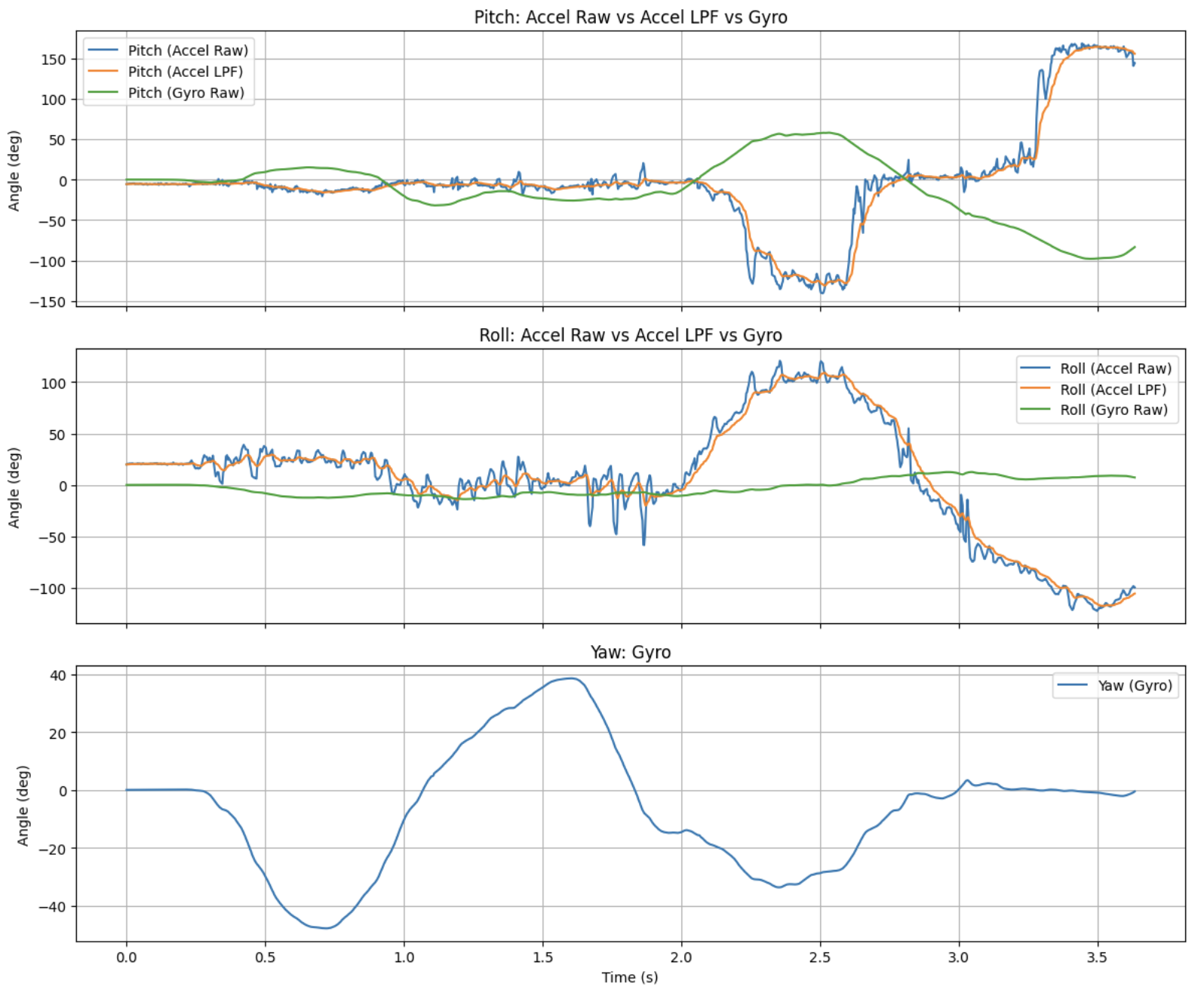
The gyroscope provides smooth motion tracking and can handle fast changes well, but because it relies on additive integration any and all small errors increase in size over time. When compared to the accelerometer which does not experience any drifting bias, the accelerometer is much more susceptible to vibrational and environmental noise. Thus, the accelerometer provides long term absolute orientation with the help of gravity and the gyroscope provides smooth tracking and accurate short term tracking.

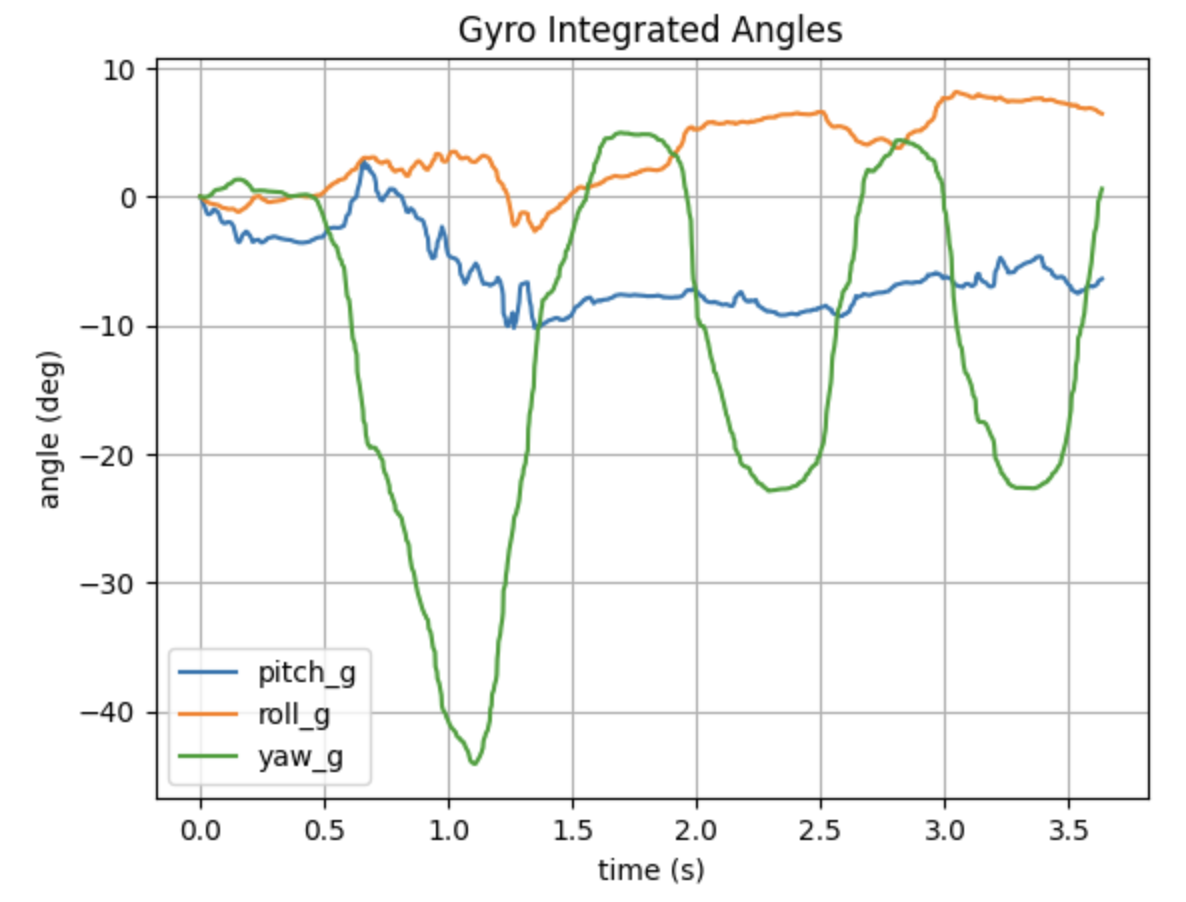
The sampling rate directly impacts the gyroscope integration quality because smaller steps provide higher resolution. When sampling is slow, each update covers a large time delta so any bias or noise encountered in this period is magnified in the sample. On the flip side, as sampling is fast, time delta decreases and integration becomes smoother and more stable.

To combine strengths of both sensors I apply a complimentary filter as follows:

angle = (1 - alpha) * (prev_angle + gyro_delta) + alpha * accel_angle;

Because my sampling rate is generally high in the range of 250-350 Hz the gyroscope actually provides the most accurate data in the near term and thus I chose to essentially weigh it at 95% with an alpha of 0.05. This means the accelerometer only lightly contributes to the total trend, but consistently counters the long term drift. With this combination the complimentary filter is able to accurately chase both stable and sporadic movements, though it does experience some lag in terms of updating.

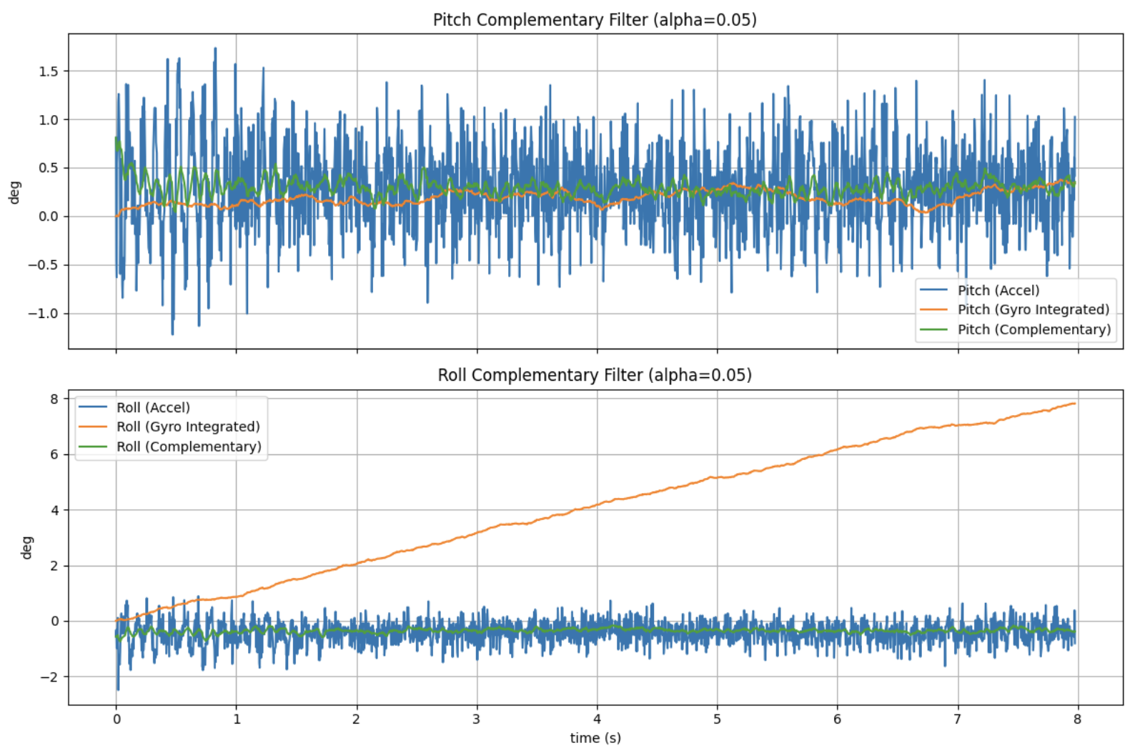
While stationary the complimentary filter is able to most accurately model the lack of movement in comparison to both the filtered accelerometer and the raw gyroscope data. While moving it is also able to accurately track the changes, most notably in the roll graph where the primary movement was occurring about the axis.

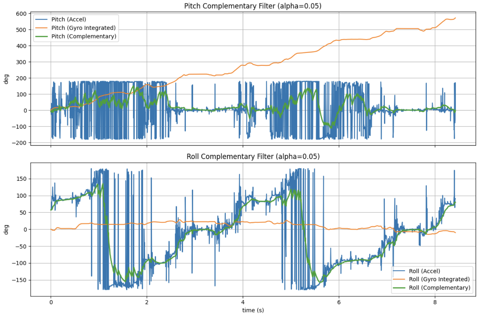
Sample Data Collection

Loop optimization

In order to increase the sampling rate I removed any delay, print, or busy wait functions to prevent unnecessary time gates. The data is stored in a predefined data array of floats. I chose a size of 2000 elements to appropriately capture over 5 seconds of data with leeway for starting and ending a motion. The IMU data collection and the bluetooth data transmit were both moved into the main loop as opposed to a specific case using data flags. So now the GET_ACC_GYRO case just resets flags as appropriate to enable the data collection in main. With these changes the mean sampling rate became 275Hz and the median was 333.3Hz, an improvement from before. At this point the IMU refresh rate is a limiting factor as the loop to collect data depends on the IMU registering containing new and available data.

In order to store data into the arrays my code first checks to see if there is new available data. If there is, it records the current time in microseconds and uses the previous time to calculate the time delta for the gyroscope integration. Gyroscope pitch roll and yaw are then respectively calculated and then stored into the respective array at the correct index. Simultaneously, the time stamp is saved using milliseconds and the data for the accelerometer’s pitch and roll are calculated and stored respectively. Then the IMU array index is incremented and the loop will wait until the data function is called again and data is available. If the data arrays are full the flag for data collection is lowered and the flag for data transmission is raised handing off responsibilities to a transmit function in the main loop.

The transmit function behaves very similarly to those in previous labs involving clearing the transmit string data, appending new information, and then finally writing the finished value. This occurs in a loop through each index as it is iterated each time and finishes upon completing the array.

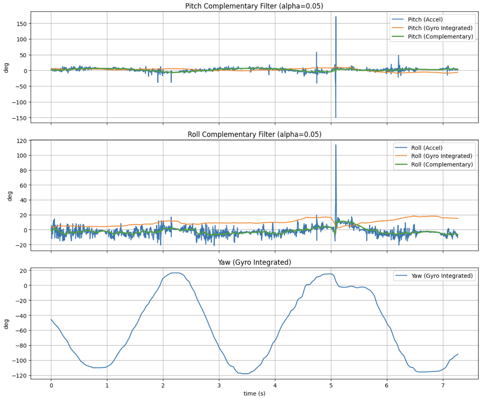
The float type was chosen for the data arrays given that the IMU outputs decimal numbers and because they take up half of the space as a double. This also provided sufficient precision for the car’s needs.

The Artemis Nano has about 384 kB of RAM available and each IMU sample as designed in my lab consists of six values: time, accelerometer pitch, accelerometer roll, gyroscope pitch, gyroscope roll, and gyroscope yaw. Each of these values are stored as 4 byte floats meaning each time sample has 24 bytes of data. At the measured sampling rate of 275Hz, the Artemis could store approximately 60 full seconds of data.

RC Car Stunt

After playing around with the car I discovered that driving the car quickly forward or backward and suddenly switching directions provided reliable torque that could flip the vehicle over to the underside. This is the stunt that I chose to record in my demonstration.